Fitting experimental data
Impedance spectroscopy data can be processed
using impedancefitter.fitter.Fitter.
Currently, a few fileformats can be used.
They are summarized in impedancefitter.utils.available_file_format().
In this example, artificial data will be generated and fitted.
We want to fit a user-defined circuit, which reads
model = 'R_s + parallel(R_ct + W, C)'
First the data is generated using the following parameters
frequencies = numpy.logspace(0, 8)
Rct = 100.
Rs = 20.
Aw = 300.
C0 = 25e-6
Then the model is defined and data generated and exported
lmfit_model = impedancefitter.get_equivalent_circuit_model(model)
Z = lmfit_model.eval(omega=2. * numpy.pi * frequencies,
                     ct_R=Rct, s_R=Rs,
                     C=C0, Aw=Aw)
data = {'freq': frequencies, 'real': Z.real,
        'imag': Z.imag}
# write data to csv file
df = pandas.DataFrame(data=data)
df.to_csv('test.csv', index=False)
The fitter is initialized with verbose output. Also, the fit results will be plotted immediately.
fitter = impedancefitter.Fitter('CSV', LogLevel='DEBUG', show=True)
os.remove('test.csv')
We use the Randles circuit that corresponds to the custom circuit model. The initial guess is passed in a dictionary with minimal information.
model = 'Randles'
parameters = {'Rct': {'value': 3. * Rct},
              'Rs': {'value': 0.5 * Rs},
              'C0': {'value': 0.1 * C0},
              'Aw': {'value': 1.2 * Aw}}
Then the fit is simply run by
fitter.run(model, parameters=parameters)
circuit: Randles
Created composite model Model(Z_randles)
Using provided parameter dictionary.
Setting values for parameters ['Rct', 'Rs', 'Aw', 'C0']
Parameters: {'Rct': {'value': 300.0}, 'Rs': {'value': 10.0}, 'C0': {'value': 2.5e-06}, 'Aw': {'value': 360.0}}
Rct needs to be positive. Changed your min value to 0.
Rs needs to be positive. Changed your min value to 0.
Aw needs to be positive. Changed your min value to 0.
C0 needs to be positive. Changed your min value to 0.
Number of data sets:1
Going to fit
#################################
fit data to Z_randles model
#################################
#########
Fitting started
#########
/home/docs/checkouts/readthedocs.org/user_builds/impedancefitter/envs/stable/lib/python3.10/site-packages/uncertainties/core.py:1024: UserWarning: Using UFloat objects with std_dev==0 may give unexpected results.
  warn("Using UFloat objects with std_dev==0 may give unexpected results.")
[[Model]]
    Model(Z_randles)
[[Fit Statistics]]
    # fitting method   = least_squares
    # function evals   = 45
    # data points      = 100
    # variables        = 4
    chi-square         = 3.4135e-21
    reduced chi-square = 3.5558e-23
    Akaike info crit   = -5165.17081
    Bayesian info crit = -5154.75012
    R-squared          = np.complex128(1-3.9947019441325314e-27j)
[[Variables]]
    Rct:  100.000000 +/- 3.0609e-12 (0.00%) (init = 300)
    Rs:   20.0000000 +/- 9.7879e-13 (0.00%) (init = 10)
    Aw:   300.000000 +/- 8.7402e-12 (0.00%) (init = 360)
    C0:   2.5000e-05 +/- 1.3554e-18 (0.00%) (init = 2.5e-06)
[[Correlations]] (unreported correlations are < 0.100)
    C(Rct, Aw) = -0.6563
    C(Rct, C0) = +0.3538
    C(Rs, C0)  = +0.3480
    C(Aw, C0)  = -0.3408
    C(Rct, Rs) = -0.1826
Solver message: `gtol` termination condition is satisfied.
Fit successful
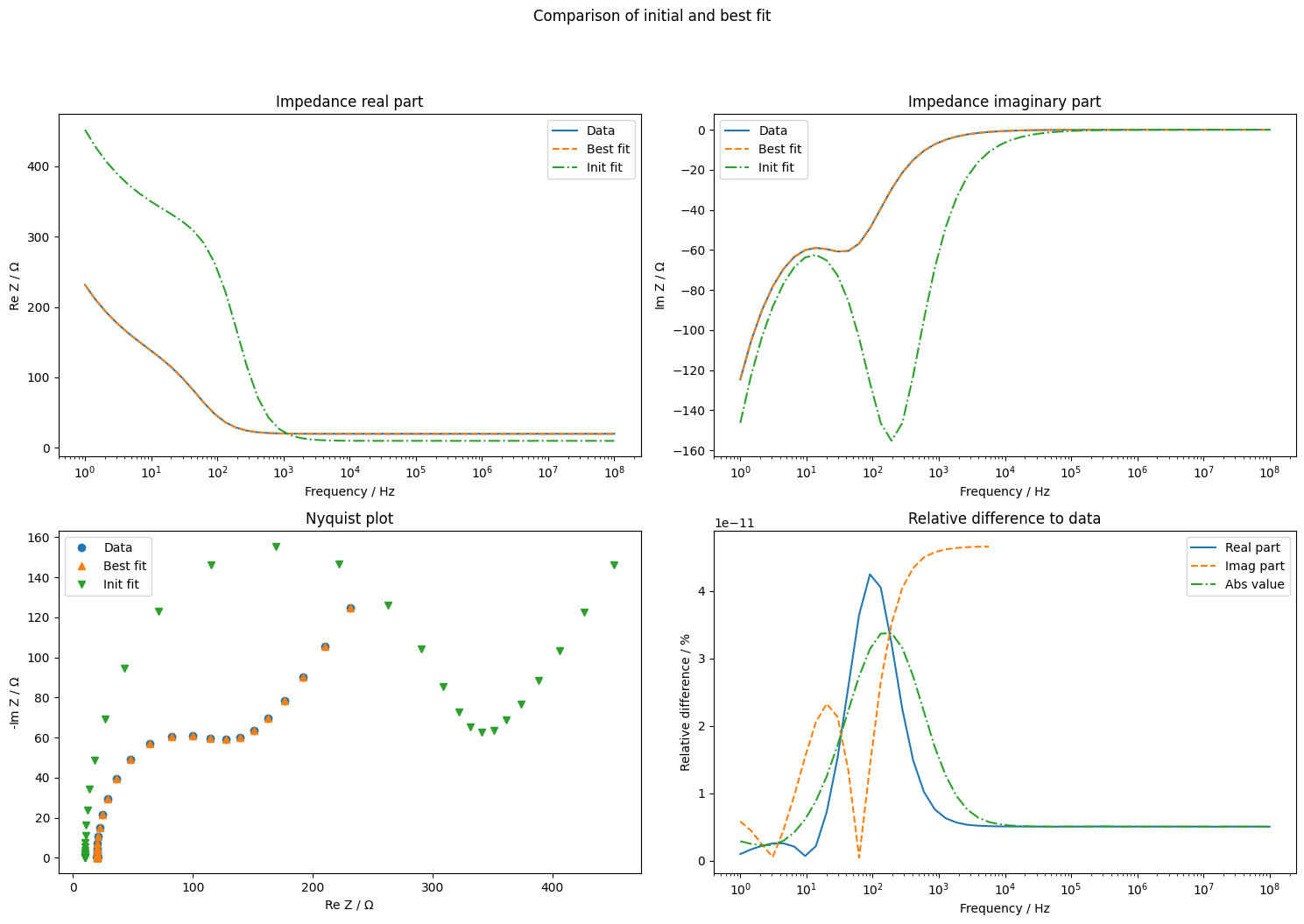
Initial and best fit can be plotted together to improve on the initial parameter guess
fitter.plot_initial_best_fit()
Here, the initial guess was passed in a dictionary with minimal information. One could also specify bounds or fix a parameter.
For example, if Rct was restricted to be between 50 and 500 and C0 was known and thus fixed, the parameters would read
parameters = {'Rct': {'value': 3. * Rct,
                      'min': 50,
                      'max': 500},
              'Rs': {'value': 0.5 * Rs},
              'C0': {'value': C0, 'vary': False},
              'Aw': {'value': 1.2 * Aw}}