Generating and using a model
The general idea of ImpedanceFitter is to generate equivalent-circuit models from the basic elements. However, there are some more complex circuits and models that are pre-implemented. One example is the Randles circuit.
The Randles circuit can be formulated in ImpedanceFitter as:
model = 'R_s + parallel(R_ct + W, C)'
The model consists of the basic elements R, W, and C with respective suffix.
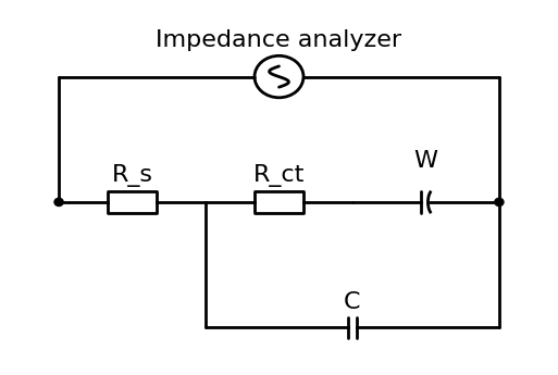
It can be drawn by
impedancefitter.draw_scheme(model)
Note that the interface to draw the equivalent circuit is quite simplistic and might not be correct for very complicated circuits!
For this circuit it yields
The impedance for a list of frequencies can the be computed by calling
frequencies = numpy.logspace(0, 8)
Rct = 100.
Rs = 20.
Aw = 300.
C0 = 25e-6

 model = 'R_s + parallel(R_ct + W, C)'
lmfit_model = impedancefitter.get_equivalent_circuit_model(model)
Z = lmfit_model.eval(omega=2. * numpy.pi * frequencies,
                     ct_R=Rct, s_R=Rs,
                     C=C0, Aw=Aw)
The same circuit has been pre-implemented and is available as
model = 'Randles'
lmfit_model = impedancefitter.get_equivalent_circuit_model(model)
Z = lmfit_model.eval(omega=2. * numpy.pi * frequencies,
                      Rct=Rct, Rs=Rs,
                      C0=C0, Aw=Aw)
Note
LMFIT names parameters with a prefix. When writing equivalent circuits, it is usual to use suffixes. Hence, the models here are formulated using suffixes but the parameters need to be named with prefixes. Then, if the model is R_ct, the respective parameter is ct_R.
Warning
Make sure to add suffixes to each element or circuit if there any elements with the same name! LMFIT does not (yet) support models, where you have for example ct_R and R. As shown here you need s_R AND (!) ct_R.
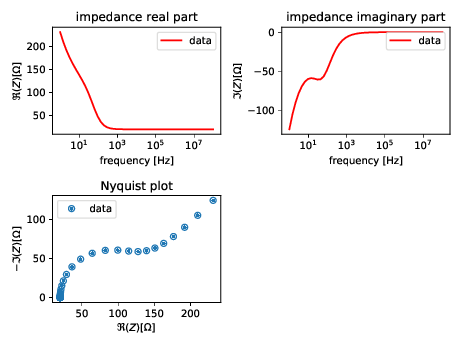
The computed impedance can also be visualized
impedancefitter.plot_impedance(2. * numpy.pi * frequencies, Z)
The real and imaginary part are shown together with the Nyquist plot