Analysing a larger data set

When performing multiple measurements on different samples, it is convenient to analyse the statistics of the data set.

Here, we show how to fit many samples and subsequently generate histograms and find the best probabality distribution to describe the data.

#    The ImpedanceFitter is a package to fit impedance spectra to
#    equivalent-circuit models using open-source software.
#
#    Copyright (C) 2018, 2019 Leonard Thiele, leonard.thiele[AT]uni-rostock.de
#    Copyright (C) 2018, 2019, 2020 Julius Zimmermann,
#                                   julius.zimmermann[AT]uni-rostock.de
#
#    This program is free software: you can redistribute it and/or modify
#    it under the terms of the GNU General Public License as published by
#    the Free Software Foundation, either version 3 of the License, or
#    (at your option) any later version.
#
#    This program is distributed in the hope that it will be useful,
#    but WITHOUT ANY WARRANTY; without even the implied warranty of
#    MERCHANTABILITY or FITNESS FOR A PARTICULAR PURPOSE.  See the
#    GNU General Public License for more details.
#
#    You should have received a copy of the GNU General Public License
#    along with this program.  If not, see <https://www.gnu.org/licenses/>.

import os
from collections import OrderedDict

import numpy as np
import pandas as pd
from impedancefitter import Fitter, PostProcess, get_equivalent_circuit_model
from matplotlib import rcParams

rcParams["figure.figsize"] = [20, 10]

# parameters
f = np.logspace(1, 8)
omega = 2.0 * np.pi * f
R = 1000.0
C = 1e-6

data = OrderedDict()
data["f"] = f

samples = 1000

model = "parallel(R, C)"
m = get_equivalent_circuit_model(model)
# generate random samples
for i in range(samples):
    Ri = 0.05 * R * np.random.randn() + R
    Ci = 0.05 * C * np.random.randn() + C

    Z = m.eval(omega=omega, R=Ri, C=Ci)
    # add some noise
    Z += np.random.randn(Z.size)

    data["real" + str(i)] = Z.real
    data["imag" + str(i)] = Z.imag

# save data to file
pd.DataFrame(data=data).to_csv("test.csv", index=False)

# initialize fitter
# LogLevel should be WARNING; otherwise there
# will be a lot of output


fitter = Fitter("CSV", LogLevel="WARNING")
os.remove("test.csv")
parameters = {"R": {"value": R}, "C": {"value": C}}
fitter.run(model, parameters=parameters)

postp = PostProcess(fitter.fit_data)
# show histograms
postp.plot_histograms()

# compare different algorithms to find matching model
print(
    "BIC best model for R:", postp.best_model_bic("R", ["Normal", "Beta", "Gamma"])[0]
)
print(
    "Chisquared best model for R:",
    postp.best_model_chisquared("R", ["Normal", "Beta", "Gamma"])[0],
)
print(
    "Kolmogorov best model for R:",
    postp.best_model_kolmogorov("R", ["Normal", "Beta", "Gamma"])[0],
)
print(
    "Lilliefors best model for R:",
    postp.best_model_lilliefors("R", ["Normal", "Beta", "Gamma"])[0],
)
print(f"Expected result:\nNormal(mu = {R}, sigma = {0.05 * R})")

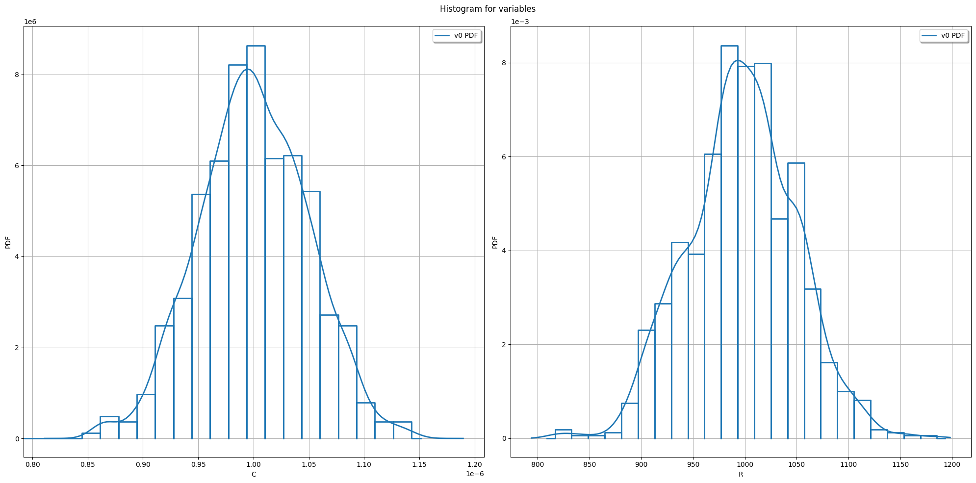
BIC best model for R: Normal(mu = 997.227, sigma = 51.7903)
Chisquared best model for R: Beta(alpha = 5.73019, beta = 5.97725, a = 816.463, b = 1185.78)
Kolmogorov best model for R: Normal(mu = 0, sigma = 1)
Lilliefors best model for R: Normal(mu = 997.227, sigma = 51.7903)
Expected result:
Normal(mu = 1000.0, sigma = 50.0)

Analysing a larger data set

See Also