Validating the data

LinKK test

Before fitting the experimental data to an equivalent circuit model, you can make sure that the data are valid. The data are valid if the real and imaginary part are related through the Kramers-Kronig (KK) relations. The LinKK test [Schoenleber2014] permits to validate the data by fitting the data to a KK compliant model. A less automated version of this test is also used in proprietary software (see, e.g. this application note).

Here, it is summarized how the test works in ImpedanceFitter.

Assume the model discussed in [Schoenleber2014]. It can be represented in ImpedanceFitter by

model = 'R_s1 + parallel(C_s3, R_s2)  + parallel(R_s4, W_s5)'

After having generated artifical data stored in test.csv, we can initialize the fitter.

fitter = impedancefitter.Fitter('CSV')

Then, the LinKK test can be performed for all data sets by running

results, mus, residuals = fitter.linkk_test()

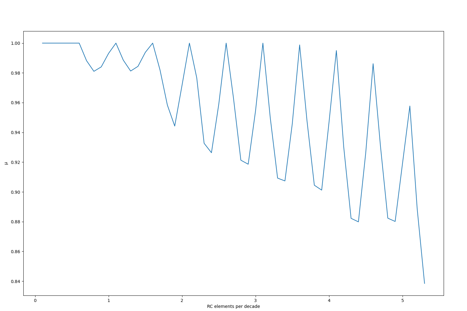
results contains the fit results as a dictionary. mus is a dictionary with all \(\mu\) values for an increasing number of RC-elements used in the LinKK-test. residuals is a dictionary containing all residuals during the least-squares fit.

The result of the fit looks like this:

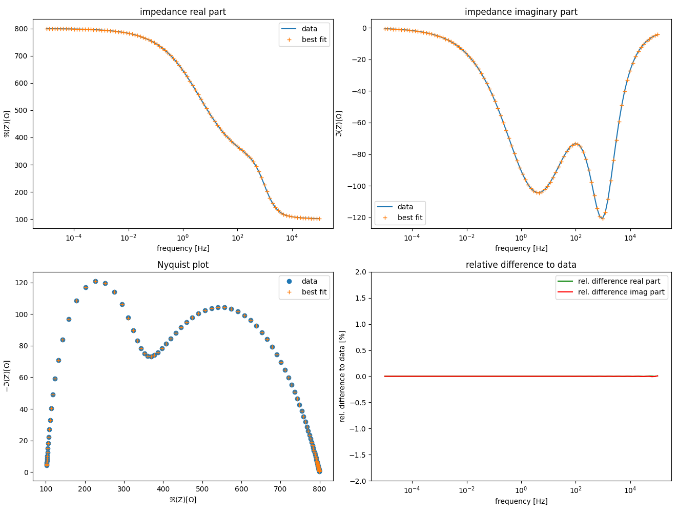
The parameter \(\mu\) decays with an increased number of RC elements as described in [Schoenleber2014]. It is used to detect overfitting. The threshold for overfitting is set to 0.85 but can be manually adjusted.

In this example, all residuals are very small (as expected for artifical data). If the relative difference exceeds 1% or if there is a drift in the residuals, concerns about the validity of the experimental data could be raised. If you observe sinusoidal oscillations in your residuals, increase the number of RC-elements either manually or by decreasing the threshold to values below 0.85. This happens when there are not many time constants are present in the impedance data. Such an example can be found in the linkk_oneRC.py example linked below.

If there is an inductive or capacitive element present, it can be benefitial to add an extra capacitance or inductance to the circuit. This can be done by

results, mus = fitter.linkk_test(capacitance=True)
results, mus = fitter.linkk_test(inductance=True)
results, mus = fitter.linkk_test(capacitance=True, inductance=True)

Especially if you observe large residuals at high frequencies, an inductive element should be added.

Numerical Integration

The Kramers-Kronig relations are integral transforms. These integrals can be evaluated numerically [Urquidi1990]. This functionality is available through the function KK_integral_transform. For the abovementioned model it can be done by

ZKK = impedancefitter.KK_integral_transform(2. * numpy.pi * frequencies, Z)
# add the high frequency impedance to the real part
ZKK += Z[-1].real
# plot the impedance and show the residual
impedancefitter.plot_impedance(2. * numpy.pi * frequencies, Z, Z_fit=ZKK,
                               residual="absolute", labels=["Data", "KK transform", ""])

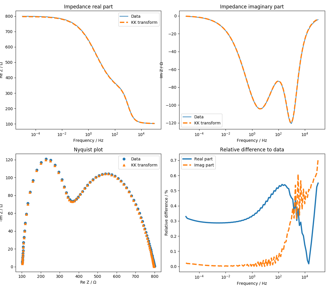
The result indicates that the data fulfil the KK relations. However, the error is not as small as with the LinKK test (mostly due to numerical accuracy of the integration scheme).

Validating the data

LinKK test

Numerical Integration

See Also